Entropy Balancing

原理と実装

Author

ネコノミスト

Published

July 3, 2025

本ファイルは，chatgpt支援のもと，シミュレーションデータを用いてエントロピーバランシングを実装してみる．

1 エントロピーバランシングの定式化

目的関数

エントロピーを最大化するようなwを見つけたい

ここでいうエントロピーとは情報理論におけるエントロピー，情報エントロピーのことであり，確率変数が持つ情報の量をさす．

エントロピーは以下の式で与えられる \[ H(w) = -\sum_{i = 1}^{n_0}w_i \log w_i \] 左辺のエントロピーを最大化するような確率変数wは，右辺を最小化するような確率変数wということである．よって，以下の目的関数を考えれば良い．

\[ \min_w \sum_{i = 1}^{n_0}w_i \log w_i \]

エントロピーを最大化するようなwに対して，3つ制約を課す

制約条件
- 1. モーメント一致 \[ \sum_{i = 1}^{ n_0 } w_i X_{ ij } = \bar{ X }_j^{ (T = 1) } \qquad \forall j \]
確率変数wは統制群の個体間では異なるが，変数間では共通である．よって，少ない個体で，変数が多い，というような状況では，モーメント一致を満たすwが存在しないかもしれない．
- 1. 正規化
\[ \sum_{ i = 1 }^{ n_0 } w_i= 1 \]
- 1. 非負制約 \[ w_i \ge 0 \]

おそらく，本命はモーメント一致であり，この制約を満たす確率変数wののうちから，エントロピーが最大なwを採用する，といった感じだろうか．最大エントロピー原理によって正当化される気がする．つまり，制約のもとで最もエントロピー（＝不確実性が高い）ものを採用することは，制約以外の異物，エコノメ風にいうならバイアス，が入ってないので，そのような確率変数wが最も妥当である．

2 ebal packageによる実装

データ生成とバランシング

library(ebal)

##
## ebal Package: Implements Entropy Balancing.

## See http://www.stanford.edu/~jhain/ for additional information.

# データ生成（再掲）
set.seed(123)
n <- 500
X1 <- rnorm(n)
X2 <- rbinom(n, 1, 0.5)
X3 <- runif(n)
logit_p <- 0.5 * X1 - 0.8 * X2 + 0.3 * X3
p <- 1 / (1 + exp(-logit_p))
treatment <- rbinom(n, 1, p)
df <- data.frame(X1, X2, X3, treatment)

# 共変量マトリクス
X_all <- as.matrix(df[, c("X1", "X2", "X3")])
Treatment <- df$treatment  # 0=control, 1=treated

# 実行：対照群を処置群に一致させる重みを学習
eb <- ebalance(Treatment = Treatment, X = X_all)

Converged within tolerance

# 検証：処置群平均
treated_mean <- colMeans(X_all[Treatment == 1, ])
# 重み付き対照群平均
weighted_control_mean <- apply(X_all[Treatment == 0, ], 2, weighted.mean, w = eb$w)
# 比較
round(treated_mean, 3)

   X1    X2    X3 
0.254 0.413 0.518

round(weighted_control_mean, 3)

   X1    X2    X3 
0.254 0.413 0.518

エントロピーで重みづけることでバランシングしたようだ．バランシングしたようだというのは正しい表現ではないようだ．そもそも制約式に，wというウェイトで平均を取ると，処置群の平均に一致する問い条件がある．これこそまさにバランシングさせてるに等しい．wでバランシングするのはなぜか，という問いの答えは，バランシングするように計算されたのがwだから，である．

out come

# アウトカムの生成（真のτ = 2）
set.seed(123)
epsilon <- rnorm(n, 0, 1)
Y <- 2 * treatment + 0.3 * X1 - 0.5 * X2 + 0.2 * X3 + epsilon
df$Y <- Y


# 処置群の平均
Y_treated <- mean(df$Y[Treatment == 1])
# 重み付き対照群の平均
Y_control_weighted <- weighted.mean(df$Y[Treatment == 0], w = eb$w)

# ATT = 処置群平均 - 重み付き対照群平均
ATT <- Y_treated - Y_control_weighted
cat("直接計算された ATT:", round(ATT, 3), "\n")

直接計算された ATT: 2

boot

ブートストラップによる信頼区間の構築を目指す．

# ライブラリ
library(ebal)
library(dplyr)


Attaching package: 'dplyr'

The following objects are masked from 'package:stats':

    filter, lag

The following objects are masked from 'package:base':

    intersect, setdiff, setequal, union

# 関数定義：1回のATT推定
estimate_att <- function(df) {
  X <- as.matrix(df[, c("X1", "X2", "X3")])
  Y <- df$Y
  treatment <- df$treatment

 invisible(capture.output(
    eb <- ebalance(Treatment = treatment, X = X)
  ))

  treated_mean <- mean(Y[treatment == 1])
  control_weighted_mean <- weighted.mean(Y[treatment == 0], w = eb$w)
  return(treated_mean - control_weighted_mean)
}

# ブートストラップ
set.seed(42)
B <- 500
att_boot <- replicate(B, {
  df_boot <- df[sample(1:nrow(df), replace = TRUE), ]
  tryCatch(estimate_att(df_boot), error = function(e) NA)
})


# 結果
boot_ci <- quantile(att_boot, probs = c(0.025, 0.975), na.rm = TRUE)
cat("ATT 推定値のブートストラップ95%信頼区間：", round(boot_ci, 3), "\n")

ATT 推定値のブートストラップ95%信頼区間： 1.998 2

3 Weight packageによる実装

データ生成

# --- パッケージの読み込み ---
library(WeightIt)
library(cobalt)   # バランスチェック

 cobalt (Version 4.6.0, Build Date: 2025-04-15)

library(survey)   # 信頼区間推定

Loading required package: grid

Loading required package: Matrix

Loading required package: survival


Attaching package: 'survey'

The following object is masked from 'package:WeightIt':

    calibrate

The following object is masked from 'package:graphics':

    dotchart

# --- データ生成（ATE = 2） ---
set.seed(123)
n <- 1000
X1 <- rnorm(n)
X2 <- rbinom(n, 1, 0.5)
pscore <- plogis(0.5 * X1 - 0.7 * X2)
treat <- rbinom(n, 1, pscore)

y0 <- 1 + 0.5 * X1 - 0.3 * X2 + rnorm(n)
y1 <- y0 + 2
y <- ifelse(treat == 1, y1, y0)
dat <- data.frame(y, treat, X1, X2)

TEの計算

# --- ATE, ATT, ATCごとの重み計算 ---
w_ate <- weightit(treat ~ X1 + X2, data = dat, method = "ebal", estimand = "ATE")
w_att <- weightit(treat ~ X1 + X2, data = dat, method = "ebal", estimand = "ATT")
w_atc <- weightit(treat ~ X1 + X2, data = dat, method = "ebal", estimand = "ATC")

# --- 重み付きデザインの作成 ---
des_ate <- svydesign(ids = ~1, weights = ~w_ate$weights, data = dat)
des_att <- svydesign(ids = ~1, weights = ~w_att$weights, data = dat)
des_atc <- svydesign(ids = ~1, weights = ~w_atc$weights, data = dat)

# --- 回帰モデルによる推定（y ~ treat） ---
fit_ate <- svyglm(y ~ treat, design = des_ate)
fit_att <- svyglm(y ~ treat, design = des_att)
fit_atc <- svyglm(y ~ treat, design = des_atc)

#計算結果
cat("ATE 推定値と信頼区間:\n")

ATE 推定値と信頼区間:

print(summary(fit_ate))


Call:
svyglm(formula = y ~ treat, design = des_ate)

Survey design:
svydesign(ids = ~1, weights = ~w_ate$weights, data = dat)

Coefficients:
            Estimate Std. Error t value Pr(>|t|)    
(Intercept)  0.84065    0.04550   18.48   <2e-16 ***
treat        1.98743    0.07342   27.07   <2e-16 ***
---
Signif. codes:  0 '***' 0.001 '**' 0.01 '*' 0.05 '.' 0.1 ' ' 1

(Dispersion parameter for gaussian family taken to be 1.164528)

Number of Fisher Scoring iterations: 2

cat("\nATT 推定値と信頼区間:\n")


ATT 推定値と信頼区間:

print(summary(fit_att))


Call:
svyglm(formula = y ~ treat, design = des_att)

Survey design:
svydesign(ids = ~1, weights = ~w_att$weights, data = dat)

Coefficients:
            Estimate Std. Error t value Pr(>|t|)    
(Intercept)  1.02444    0.05305   19.31   <2e-16 ***
treat        1.99661    0.07648   26.11   <2e-16 ***
---
Signif. codes:  0 '***' 0.001 '**' 0.01 '*' 0.05 '.' 0.1 ' ' 1

(Dispersion parameter for gaussian family taken to be 1.163522)

Number of Fisher Scoring iterations: 2

cat("\nATC 推定値と信頼区間:\n")


ATC 推定値と信頼区間:

print(summary(fit_atc))


Call:
svyglm(formula = y ~ treat, design = des_atc)

Survey design:
svydesign(ids = ~1, weights = ~w_atc$weights, data = dat)

Coefficients:
            Estimate Std. Error t value Pr(>|t|)    
(Intercept)  0.71376    0.04431   16.11   <2e-16 ***
treat        1.98070    0.07880   25.14   <2e-16 ***
---
Signif. codes:  0 '***' 0.001 '**' 0.01 '*' 0.05 '.' 0.1 ' ' 1

(Dispersion parameter for gaussian family taken to be 1.154199)

Number of Fisher Scoring iterations: 2

バランスチェック

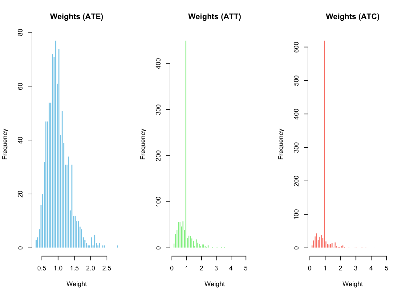
par(mfrow = c(1, 3))  # 1行3列に分割表示

hist(w_ate$weights,
     breaks = 50,
     main = "Weights (ATE)",
     xlab = "Weight", col = "skyblue", border = "white")

hist(w_att$weights,
     breaks = 50,
     main = "Weights (ATT)",
     xlab = "Weight", col = "lightgreen", border = "white")

hist(w_atc$weights,
     breaks = 50,
     main = "Weights (ATC)",
     xlab = "Weight", col = "salmon", border = "white")

par(mfrow = c(1, 1))  # レイアウトを戻す

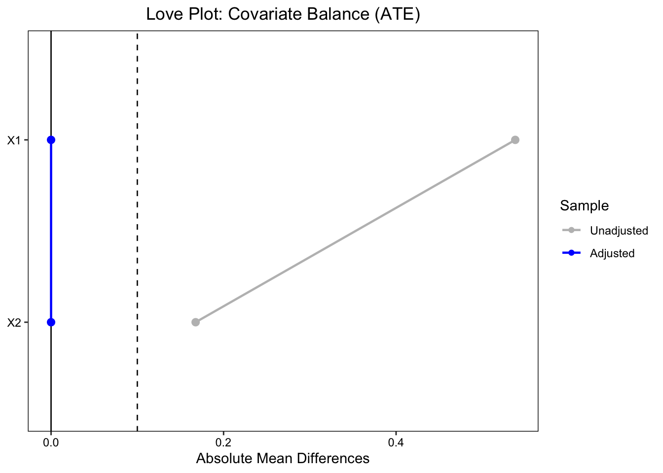
# ATE
love.plot(w_ate,
          stat = "mean.diffs", abs = TRUE, thresholds = c(m = .1),
          var.order = "unadjusted", line = TRUE,
          title = "Love Plot: Covariate Balance (ATE)",
          colors = c("grey", "blue"))

Warning: Standardized mean differences and raw mean differences are present in
the same plot. Use the `stars` argument to distinguish between them and
appropriately label the x-axis. See `?love.plot` for details.

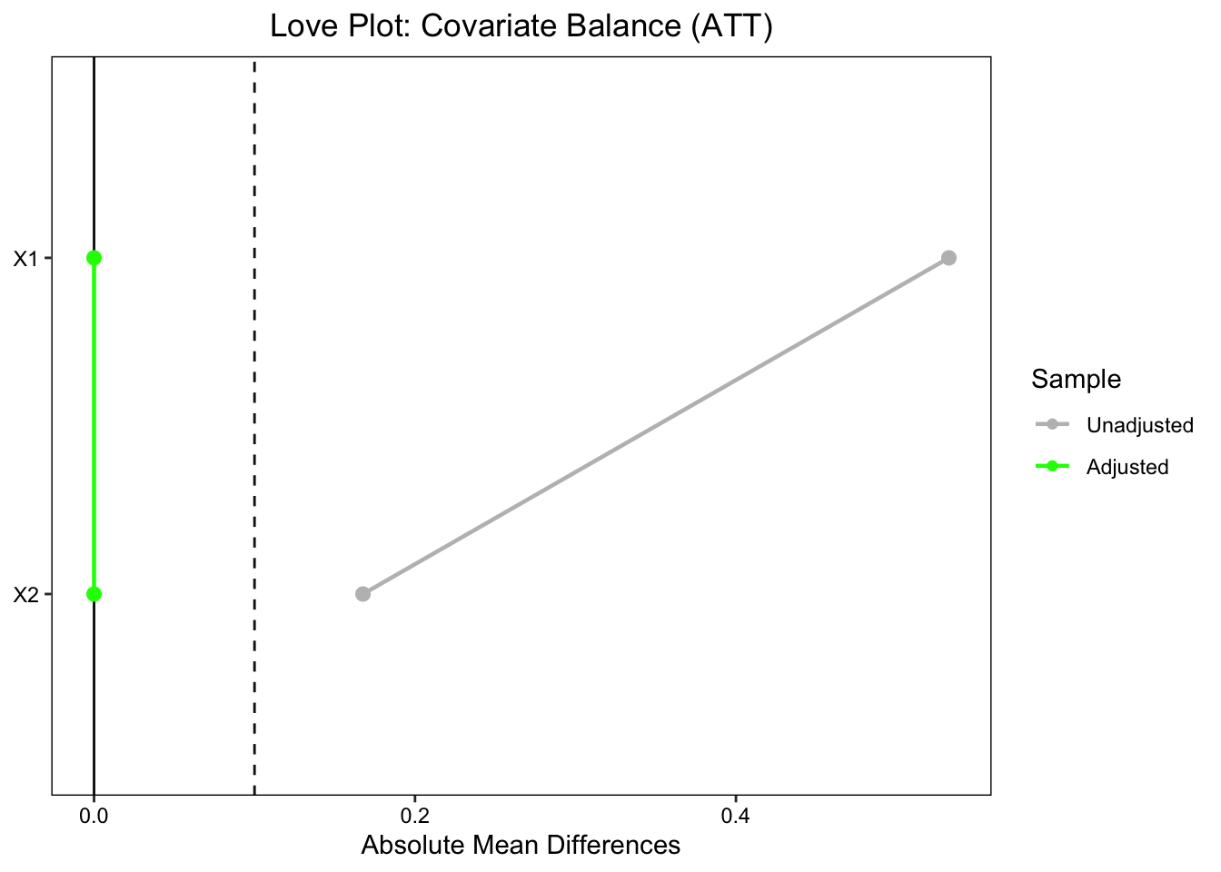
# ATT
love.plot(w_att,
          stat = "mean.diffs", abs = TRUE, thresholds = c(m = .1),
          var.order = "unadjusted", line = TRUE,
          title = "Love Plot: Covariate Balance (ATT)",
          colors = c("grey", "green"))

Warning: Standardized mean differences and raw mean differences are present in
the same plot. Use the `stars` argument to distinguish between them and
appropriately label the x-axis. See `?love.plot` for details.

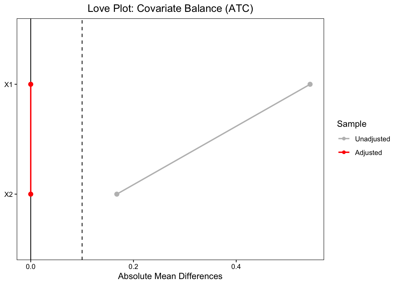
# ATC
love.plot(w_atc,
          stat = "mean.diffs", abs = TRUE, thresholds = c(m = .1),
          var.order = "unadjusted", line = TRUE,
          title = "Love Plot: Covariate Balance (ATC)",
          colors = c("grey", "red"))

Warning: Standardized mean differences and raw mean differences are present in
the same plot. Use the `stars` argument to distinguish between them and
appropriately label the x-axis. See `?love.plot` for details.

4 DiD

エントロピーバランシングによる重み付けをしたうえで，DiDを実装してみる． 2 by 2で考えてみよう．

model

\[ Y_{it} = \alpha + \delta \cdot Post_t + \tau \cdot Treat_i + \beta \cdot(Post_t \times Treat_i) + \varepsilon_{it} \]

データ生成

# パッケージの読み込み
library(ebal)
library(survey)

# 再現性確保
set.seed(123)

# サンプル数
n <- 500

# 共変量（時間不変）
X1 <- rnorm(n)
X2 <- rbinom(n, 1, 0.5)
X3 <- runif(n)

# 処置群かどうか（0: control, 1: treated）
treatment <- rbinom(n, 1, 0.5)

# 時間（0: before, 1: after）
time <- rbinom(n, 1, 0.5)

# 真のDID効果：treat × time の交差項
true_effect <- 2

# アウトカム生成：線形関数 + DID効果 + 誤差項
# 基礎回帰式: y = beta0 + beta1*treat + beta2*time + beta3*treat*time + e
y <- 1 + 0.5*treatment + 1.5*time + true_effect*treatment*time +
     0.3*X1 - 0.7*X2 + 0.5*X3 + rnorm(n)

# データフレームにまとめる
df <- data.frame(X1, X2, X3, treatment, time, y)

エントロピーバランシング

# 共変量マトリクス
X_covariates <- as.matrix(df[, c("X1", "X2", "X3")])
Tr <- df$treatment  # 1 = treated, 0 = control

# エントロピーバランシング：control を reweight
eb <- ebalance(Treatment = Tr, X = X_covariates)

Converged within tolerance

# 重みを df に追加（treated=1には重み1, controlにはeb$w）
df$w <- NA
df$w[df$treatment == 1] <- 1
df$w[df$treatment == 0] <- eb$w

DiD推定

# surveyパッケージのデザインオブジェクトを作成
design <- svydesign(ids = ~1, data = df, weights = ~w)

# 回帰モデル：DID形式（treatment × time 交差項）
did_model <- svyglm(y ~ treatment * time, design = design)

# 結果の表示
summary(did_model)


Call:
svyglm(formula = y ~ treatment * time, design = design)

Survey design:
svydesign(ids = ~1, data = df, weights = ~w)

Coefficients:
               Estimate Std. Error t value Pr(>|t|)    
(Intercept)     1.00294    0.09372  10.702  < 2e-16 ***
treatment       0.59123    0.14722   4.016 6.83e-05 ***
time            1.32843    0.13062  10.170  < 2e-16 ***
treatment:time  2.08285    0.19791  10.524  < 2e-16 ***
---
Signif. codes:  0 '***' 0.001 '**' 0.01 '*' 0.05 '.' 0.1 ' ' 1

(Dispersion parameter for gaussian family taken to be 1.211858)

Number of Fisher Scoring iterations: 2

正しい処置効果が推定されている．